Weighting methods

Just like matching, inverse-probability weighting (IPW) is all about improving the balance of covariates across your control and treatment groups. To understand how IPW works, we need to understand how survey sampling works.

A digression on survey sampling

Imagine we are interested in polling opinions about a specific topic in your country. Of course, you want your sample to be representative of the population. A representative sample is a subset of the population that accurately reflects the larger population’s key characteristics.

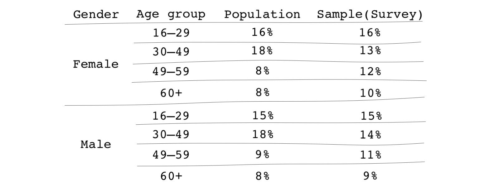
Let’s say the key demographic variables are age and gender. Suppose, for whatever reason, such as differences in survey participation across different demographic groups, your sample isn’t fully representative of the larger population. The differences are summarized in the table below.

Within the overall population, 49-59-year-old female subjects make up 8 percent of the population; however, they make up 12 percent of your sample. These types of discrepancies occur all the time in survey sampling. The remedy is straightforward. Researchers often use weighting to make the survey look similar to the general population.

This is how weighting works:

Identify key subgroups of your population and calculate the share of each subgroup out of your entire population or sample.
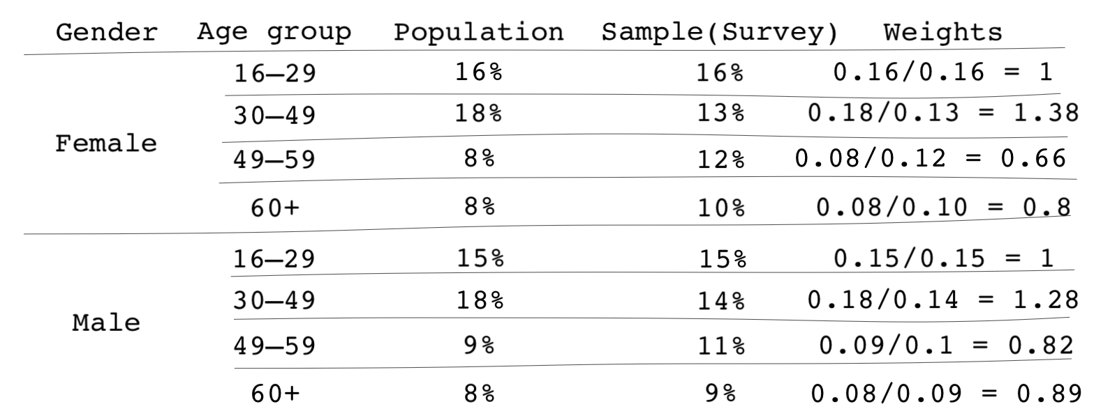
Then calculate weights using the share of the subgroup in the population divided by their share in the survey sample. For instance, for the 49-59-year-old female group we discussed above, their weight would be $0.08/0.12 = 0.67$ . The following table shows the weights for each group.

Next, instead of giving individuals in that subgroup a weight of 1, we give them a weight of 0.67. In other words, respondents in that subgroup count as roughly 2/3 of an individual because combined, they are overrepresented in the data.
Finally, if we’re doing any tabulation or analysis of the data, then we subsequently apply these weights.

Inverse-probability weighting

Now that you understand the idea behind survey weighting let’s see how Inverse-probability weighting (IPW) works. Note that you may also come across the acronym IPTW for this, which stands for inverse probability of treatment weighting. It’s the same thing! 🤨

With IPW, we’re not comparing a sample to a population. Instead, IPW is based on the idea that the share of those receiving the treatment in each subgroup of the sample

may be different than 0.5. Remember in an ideal scenario which is a randomized experiment, this share is equal to 0.5.
may also vary based on the value of the covariates. In other words, the probability of receiving the treatment may depend on the value of the covariates.

Consider an example similar to the one we saw at the start of this lesson. Here, we have categorized the number of subjects in the treatment and control groups by two covariates: gender and age group. For instance, there are 27 males aged 50-59 in the treatment group, and there are 21 individuals fitting the same description in the control group. For every subgroup in the sample, we can calculate the share of individuals who are treated.

The share of treated individuals in each group can be interpreted as the probability of receiving treatment or, as we called it before, the propensity score. For instance,

P(D=1 | \text{Gender } = \text{Female }, \text{Age Group } = \text{16-29}) = 0.4

Based on the table, the propensity scores vary from subgroup to subgroup. For instance, the probability of receiving the treatment is, in general, higher among men than women. It is also obvious that those propensity scores are mainly different than 0.5.

In IPW, similar to the basic survey sampling we saw earlier, we weight observations (in both the treatment and control) so that the share of treated subjects across all covariates is equal to 0.5.

The value of the probability of receiving treatment for women aged 16-29 means for every 4 treated subjects, there are 6 control subjects. If we weight each treated observation in the women aged 16-29-year-old category by $1/0.4$ and every control observation in that same category by $1/(1-0.4)$ , then in the weighted sample, the probability of receiving the treatment will be the same and equal to 0.5 across our sample.

In effect, we do the following for each observation $i$ :

Find the propensity score for the subject just like in matching
If the observation is in the treatment group, we weight them by $1/{\text{PS}_i}$
If the observation is in the control group, we weight them by $1/(1-\text{PS}_i)$

Because the weights are proportional to the inverse probability of receiving the treatment, the method is mainly referred to as inverse probability weighting.

What is the implication of weighting observations so that the probability of receiving treatment for all observations gets close to 0.5?

We make the treatment assignment ignorable.

We make everyone a potential for the treatment group.

SUTVA will no longer be violated.

After weighting the observations by inverse probabilities, there won’t be any confounding because covariates no longer determine the probability of receiving the treatment. If all probabilities are 0.5, it’s as if we flipped a coin to determine who receives the treatment and who doesn’t.

Again, similar to matching, IPW requires that we have already identified the covariates that satisfy the ignobility assumption

IPW versus matching

Hopefully, it’s already clear to you that propensity-score matching and inverse-probability weighting have a lot in common. First, both are based on the probability of treatment, i.e., the propensity scores.

Second, in both matching and IPW, we assign weights to observations. Matching can be thought of as giving weights of 1 or 0 to observations depending on whether they’re selected as a match or not. If a weight of 0 is given to an observation, that observation is dropped from the data. However, in IPW, the weights can theoretically be any number from zero to infinity (although, you should avoid large weight as they will distort your results).

An advantage of using IPW over matching is that it uses all observations rather than discarding some of them. So in some ways, IPW is similar to full matching or sub-classification (IPW can be thought of as sub-classification when the number of observations and subclasses go to infinity).

How is IPW done?

The steps for IPW can be summarized as follows:

estimating the propensity scores
calculating the weights for each observation based on their propensity score and treatment status
estimating the causal effects based on the weighted sample.

Estimating propensity scores is similar to what we learned in propensity-score matching. We can simply use logistic regression and the covariates that satisfy the ignorability assumption to estimate the propensity scores. Like we saw with matching, the functional form of the model that estimates the propensity scores will be irrelevant when using IPW.

We then use the weighting formula we discussed above to calculate the weights. Based on the formula, weights can be any number between 0 and infinity. However, weights that are too large add noise to our causal estimate. For instance, a weight of 1,000 that is considered too large means the observation associated with that weight is counted 1,000 times, therefore, inflating the standard errors of our estimates.

Extremely large weights can also be seen as a violation of the positivity assumption. Positivity assumption ensures that every subject in the study has some chance of receiving the treatment and the treatment assignment is not deterministic. An extremely large weight is equivalent to an extremely small propensity score, almost zero. This, therefore, violates the positivity assumption.

To check weights, we can either tabulate or plot them using summary statistics or histograms. If we observe very large weights, it can be mainly due to large values of the covariates or misspecification of the propensity-score model. If the large weight problem is due to misspecification, we should revise our propensity-score model.

However, if the problem is structural, we can trim observations with large weights. We have to be cautious about the implications of doing this. Trimming observations in causal inference changes the interpretation of causal estimates.

Another way to avoid large weights is to change our weighting formula. The weighting scheme mentioned above, i.e., weighting observations by $1/\text{PS}$ and $1/(1-\text{PS})$ is likely to create large weights.

To avoid this, other formula have been suggested. For instance, Li and Greene offer the following:

w = \dfrac{\text{min}\{\text{PS}_i, 1-\text{PS}_i\}}{\text{PS}_i D_i + (1-\text{PS}_i) (1-D_i)}

Where $D_i$ is the treatment indicator and is equal to 1 if the subject is treated and 0 if otherwise.

While the first weighting formula is shown to give the average treatment effect (ATE), the second formula shows the average treatment effect among the matchable (ATM). ATM is similar to the treatment effect for a population once we do one-to-one matching.

If we’re interested in estimating average treatment effect among the treated (ATT), we can use the following weighting formula:

w = \dfrac{\text{PS}_i D_i}{\text{PS}_i}+\dfrac{\text{PS}_i(1-D_i)}{(1-\text{PS}_i )}

Similar to matching, it’s easy to do weighting in most statistical packages. Let’s revisit Zucco’s paper on cash transfers and voter behavior 🇧🇷. First, if you don’t already have the data in your software, let’s import it again and drop the missing values.

# Importing the data from a web link
# Original dataset can be found here:
# https://dataverse.harvard.edu/dataset.xhtml?persistentId=hdl:1902.1/20257
cash_voting <- read.csv("https://bit.ly/cash_voting")

# Python codes will be added soon

* Importing the data from a web link
* Original dataset can be found here:
* https://dataverse.harvard.edu/dataset.xhtml?persistentId=hdl:1902.1/20257
import delimited https://bit.ly/cash_voting

To calculate weights, we need to specify the propensity score model. This model should include variables that satisfy the ignorability assumption, i.e., controlling for them prevents any confounding in the estimates. We can then find the weights using the following functions.

# If you don't have the package twang installed, first install it
# install.packages("twang")
# Note: You can alternatively use the package WeightIt
# Load the library for inverse-probability weighting analysis
library(twang)

# Let's first create the square version of the variable hdi_2000
# twang doesn't allow for in-formula variable creation
cash_voting$hdi_2000_sq <- (cash_voting$hdi_2000)^2

# The model below uses a weighting scheme for estimating average treament
# effect among the treated. You can use the help file for the function ps()
# by typing ?ps to see what other parameters you can adjust. 
weighted_output <- ps(beneficiary ~ female + age + yrs_school + nonwhite + growth +
                                    hdi_2000  + hdi_2000_sq + distcap + metropolitan, 
                      data=cash_voting,
                      stop.method="ks.max",
                      estimand = "ATT")

# Python codes will be added soon

* In Stata, the teffects package can estimate the weights. However, the package
* does not provide options for estimating ATT as opposed to ATE. Therefore, it's
* best to estimate the weights and the treatment effects manually.
* We first use a logit model to estimate the propensity scores
* We use a logit model because the dependent variable in the propensity
* score model is binary.
logit beneficiary female age yrs_school nonwhite growth hdi_2000 ///
c.hdi_2000#c.hdi_2000 distcap metropolitan

* Then we predict the propensity scores using `predict`
predict p_beneficiary, pr

Note that the left-hand side of the regression is the treatment variable beneficiary. The weights are now calculated. But we should check whether there are any super large weights by looking at their summary or histogram. Run the code and check the results!

# Let's store the vector of weights using the function get.weights()
# from the package twang. The get.weights() function extracts the propensity 
# score weights.
cash_voting$w <- get.weights(weighted_output, stop.method="ks.max")

# We can look at the histogram of the weight by simply using the ggplot2 package.
library(ggplot2)
ggplot(cash_voting) +
    geom_histogram(aes(x=w))

# Python codes will be added soon

* Now, let's calculate the weights
* First, we need to create an empty vector of weights
gen w=.

* Then we use the following weighting formula that we saw before
* to estimate ATT
replace w=1 if beneficiary==1
replace w=p_beneficiary/(1-p_beneficiary) if beneficiary==0

* We can look at the histogram of the weight by simply using the ggplot2 package.
hist w

Phew! No extremely large weights. So we should be good. Now, just like what we did in matching, let’s take a look at the balance of the covariates. First the balance table.

# cobalt is a package that provides balance assessment tools
# in a more visually pleasing way. It shows balances before and after 
# matching/weighting. It can be used in conjunction with the package twang 
# The output of ps() function can be used as an argument in functions from 
# the cobalt package.
library(cobalt)

# We can first see the balance tables for the covariates. 
# Function balance.tab() provides mean standardized bias after weighting.
bal.tab(weighted_output)

# Python codes will be added soon

* We need to first use the teffects ipw function to estimate the weights
* It's true that you've already done this, but in order to look at the balance
* tables, we need to first run this command
teffects ipw (voted) (beneficiary female age yrs_school nonwhite growth hdi_2000 ///
c.hdi_2000#c.hdi_2000 distcap metropolitan, logit), atet

* We can summarize the covariates by group in the unweighted 
* and weighted data
tebalance summarize

And maybe some balance plots:

# We can specify the name of the covariate we're checking for balance. 
# the function bar.plot shows the histogram or density functions of the 
# variable specified. If we specify which as both, we will see both the
# unweighted (original) and weighted samples.
# The following checks the density plots of the variable years of
# schooling
bal.plot(weighted_output, var.name = "yrs_school", which = "both")

# We can specify the threshold as 0.2 which can be seen as the 
# upper limit for a good match
love.plot(weighted_output, binary = "std", thresholds = c(m = .2))

# Python codes will be added soon

* We can specify the name of the covariate we're checking for balance. 
* the function tebalance shows the histogram or density functions of the 
* variable specified. We can check both unweighted and weighted samples.
* The following checks the density plots of the variable years of
* schooling
tebalance density yrs_school

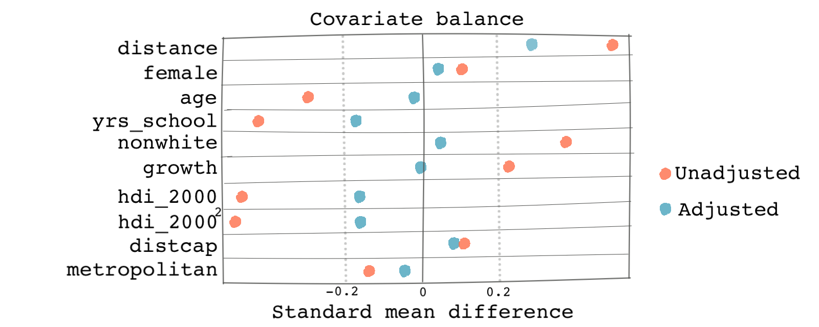
We get graphs similar to the ones below. Based on both the distribution of treatment and the Love plot, we can see that there is a better balance across the propensity scores and the covariates post-weighting.

Outcome analysis

In matching, once observations were matched, we could either simply compare the potential outcomes or run a regression with the matched data set to estimate the causal effects.

In inverse-probability weighting, estimating the causal effect is very similar. We can either calculate the average of weighted potential outcomes under treatment and under no treatment and take the difference. The mean of weighted potential outcomes under treatment are:

E(Y^1) = \dfrac{\sum_{i=1}^n {\dfrac{D_i Y_i}{\text{PS}_i}}}{\sum_{i=1}^n {\dfrac{D_i}{\text{PS}_i}}}

And the potential outcomes under no treatment are:

E(Y^0) = \dfrac{\sum_{i=1}^n {\dfrac{(1-D_i) Y_i}{(1-\text{PS}_i)}}}{\sum_{i=1}^n {\dfrac{(1-D_i)}{(1-\text{PS}_i)}}}

Note that the potential outcomes are weighted by the propensity scores. Therefore, average treatment effect is simply $E(Y^1) - E(Y^0)$ . You can see why we don’t like large weights that are associated with really small propensity scores. Tiny propensity scores inflate potential outcomes.

We can also use regression of the outcome on just the treatment to estimate the causal effect using the weighted sample instead of the original sample. However, it’s usually suggested that we include the covariates (or at least the most important ones) in the outcome model as well.

Doing regression with weights is usually simple in most statistical software. Let’s see how.

# The survey package can be used for performing outcome analysis using the weights. 
# This package is usually used for survey weighting but because of the similarities
# of inverse-probability weighting and survey weighting, it can be used for our
# application. 
library(survey)

# The function svydesign() account for the weights when computing standard error
# estimates. The weights may then be used as case weights in a svydesign 
# object. 
design.ps <- svydesign(ids=~1, weights=~w, data=cash_politics_nomiss)

# The propensity score-adjusted model can be computed with svyglm. 
# We can only include the treatment variable on the right-hand side
outcome_model1 <- svyglm(voted ~ beneficiary, design=design.ps)
summary(outcome_model1)

# Python codes will be added soon

* Finally we use the outcome model to estimate the treatment effect.
* Note that we have to feed weights to the regression formula.
* We use a logit model because the outcome variable is binary.
logit voted beneficiary [pweight=w]

The treatment effect is equal to 0.44 which means if the person is a beneficiary of the cash program, the odd ratio of voting for the incumbent party increases by 0.44. And if we include the covariates in the outcome regression model, the coefficient slightly decreases to 0.41.

# It's better to include covariates in the outcome model. 
outcome_model2 <- svyglm(voted ~ beneficiary + gender + age + yrs_school + 
                             income_cat + nonwhite + growth +
                             hdi_2000 + distcap + metropolitan, design=design.ps)
summary(outcome_model2)

# Python codes will be added soon

* It's better to include covariates in the outcome model. 
logit voted beneficiary female age yrs_school nonwhite growth hdi_2000 ///
c.hdi_2000#c.hdi_2000 distcap metropolitan [pweight=w]

Congratulations! 🎊 🎉 You have completed the module on matching and weighting methods.

In the next module, we will learn about a method that comes in handy when the ignorability assumption is violated.

Next Lesson

Back to randomized experiments

You'll learn about the basics of causal inference and why it matters in this course.

Go to the next lesson