What do DAGs tell us?

As we saw in the last lesson, DAGs can be used to map variables and make our assumptions about causal relationships more explicit. In the rest of this module, we will learn to see how this mapping process aids us in identifying confounders and knowing which variables need to be controlled for.

Let’s begin by learning how DAGs show dependence and conditional dependence between variables. For this, you’ll need to know what conditional probability and joint distributions are. If you can’t remember what these terms mean, we suggest you open your favorite basic probability book or just do a Wiki search to refresh your memory. Do that now, and we’ll meet you right back here.

Using DAGs to show conditional dependence

Alright, we know from probability, that two variables $X_1$ and $X_2$ are independent if information about one doesn’t tell you anything about the other.

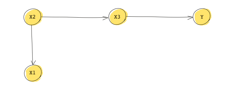
But let’s say a variable $X_1$ affects variable $Y$ through a third variable variable $X_2$. This can be easily shown using DAGs. So $X_2$ lies on the causal path from $X_1$ to $Y$.

In statistics, conditioning on a variable (or controlling for it) means that this variable is treated as being known to us (e.g. if the variable is binary, we know if it’s 0 or 1. From conditional probability, we know that in this case the conditional distribution of $Y$ given $X_1$ and $X_2$ is equal to the conditional distribution of $Y$ given only $X_2$.

Therefore, in the example above, as long as we condition on $X_2$, we don’t need $X_1$ to get the conditional distribution of $Y$. In other words:

An interpretation of the mathematical statement above is that if we condition on $X_2$, then $Y$ and $X_1$ become independent.

Based on this DAG, we know:

• $Y$ is directly affected by $X_2$ and only indirectly affected by $X_1$.
• $\Pr(Y|X_1, X_2) = \Pr(Y|X_2)$
• Also $\Pr(Y|X_1) \neq \Pr(Y)$ which means $Y$ and $X_1$ are conditionally (marginally) dependent because they’re indirectly dependent on each other. They become independent if we condition on (control for) $X_2$.
• Similarly, $\Pr(X_1|X_2, Y) = \Pr(X_1|X_2)$

Using DAGs to decompose a joint distribution

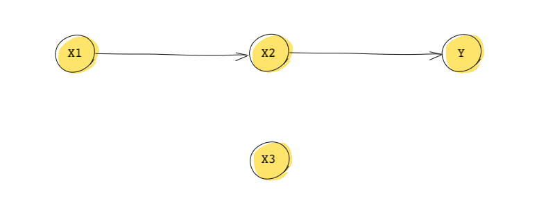
Now consider the following DAG that is similar to the one we just saw but with an additional variable:

From probability we know that the in general, $\Pr(X_1, X_2, Y)$ represents the joint distribution of $X_1$, $X_2$, and $Y$. This DAG is telling us that:

• $\Pr(X_3|X_1, X_2, Y) = \Pr(X_3)$ because $X_3$ is independent of all other variables.
• $\Pr(Y|X_1, X_2, X_3) = \Pr(Y|X_2)$
• Similarly, $\Pr(X_1|X_2, X_3, Y) = \Pr(X_1|X_2)$.

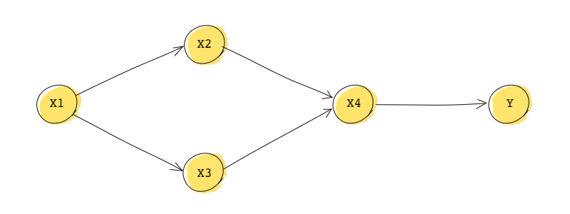
We can use DAGs to help us decompose a joint distribution (writing a joint distribution as a combination of conditional distributions). For this, we start with the roots (remember, a root = a node without any parents). Then we move from roots down to their descendants while conditioning on parents. We’ll use another DAG to see how to do this. This one is a bit more complicated:

First, this DAG tells us:

• $\Pr(X_1|X_2, X_3, Y) = \Pr(X_1|X_2)$
• $\Pr(X_2|X_1, X_3, Y) = \Pr(X_2|X_1, X_3)$
• $\Pr(Y|X_1, X_2, X_3) = \Pr(Y|X_3)$

We can also find the join distribution:

This means we can decompose the joint distribution by starting from the root $X_2$.

Practice makes perfect. Let’s look at another one. This ones a bit more involved…

Mathematically, the DAG tells us:

• $\Pr(Y|X_1, X_2, X_3, X_4) = \Pr(Y|X_4)$
• $\Pr(X_1|X_2, X_3, X_4, Y) = \Pr(X_1|X_2, X_3)$
• $\Pr(X_2|X_1, X_3, X_4, Y) = \Pr(X_2|X_1, X_4)$
• $\Pr(X_3|X_1, X_2, X_4, Y) = \Pr(X_3|X_1, X_4)$
• $\Pr(X_4|X_1, X_2, X_3, Y) = \Pr(X_4|X_2, X_3, Y)$

The joint distribution of this DAG is:

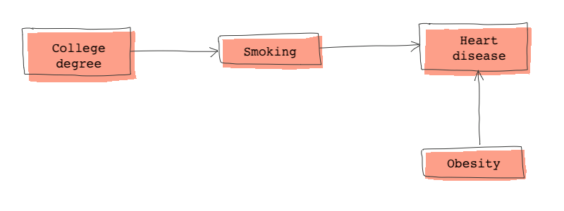
Finally, let’s forget about all those symbolic variables and talk about a more realistic DAG. Consider the DAG below:

From this DAG we know that heart disease is directly caused by obesity and smoking and indirectly caused by (not) having a college degree.

Heart disease and college degree are conditionally dependent. However, if we condition on smoking, heart disease and college degree become independent. What does this statement really mean?

The statement really means that if we control for smoking, we no longer need to control for college education. In other words, for individuals who smoke the same number of cigarettes a day, education no longer determine their chances of having a heart disease.

The DAG above also tells us the obesity is only dependent on heart disease and college degree is only dependent on smoking.

Finally the joint distribution derived from the DAG above is:

To decompose the joint distribution, we start from the two root nodes (college degree and obesity, then we move from those two roots down their descendants while conditioning on parents

To recap, a simple DAG, tells us a lot about the relationship between variables and the direction of the relationships. The relationship between DAGs and joint probability distributions are one to one. We can only derive one and only one joint distribution from a DAGs and a joint distribution can only lead to a unique DAG.