Basics of causal graphs

The most important step in estimating a causal effect in an observational study is to satisfy the ignorability assumption by identifying relevant confounders.

We had a long discussion about confounders and how to define them. But we also said that the common-cause criteria are not the most accurate way to identify confounders. In this module, we will see how causal graphs can help us with that.

What are causal graphs?

So far, we’ve used mathematical notation and words to communicate causal relationships among variables. For example, we have said $X_1$ can affect $Y$ and $X_2$ can affect both $X_1$ and $Y$.

This simple sentence dictates the causal relationship among $X_1$, $X_2$, and $Y$. If the number of variables is large and especially when the relationship among variables is complex, describing the relationship between variables with words may not be the best idea.

As an alternative, we use causal graphs, or what we usually call directed acyclic graphs (DAGs). DAGs provide a more intuitive language for communicating the dynamics of causality. The idea is very simple.

When we think a variable $X_1$ is the cause of the variable $Y$, we simply draw an arrow going from $X_1$ to $Y$.

These diagrams are called directed graphs because of the arrows. The arrows indicate the presence and the direction of a causal relationship.

They are called acyclic because there are no closed paths. We’ll see what this means in a minute, but first, we need to introduce a few more terms.

In the graph above, $X_1$ and $Y$ are called nodes. You can think of the nodes as representing the random variables we’ve been working with so far. The arrow that connects the nodes is called an edge or sometimes a link. Nodes that are connected by a single edge are called adjacent nodes. In the DAG above $X_1$ and $Y$ are adjacent nodes.

Most DAGs consist of more than two nodes and one edge. In cases such as these, we use the term path to describe a sequence of edges, where a node that ends one edge begins the next edge in the sequence.

We can further differentiate between direct and indirect paths. Consider the causal effect of video games on obesity. Playing video games does not directly lead to obesity (as there’s no medical evidence of a direct link). However, playing a lot of video games can lead to less exercise which may then lead to obesity. In this scenario, the path between video games and obesity is an indirect path the path between these nodes passes through a third node, “exercise.”

The path between the video game node and the exercise node is a direct path. There are no intermediate nodes between them.

Let’s take a look at another DAG.

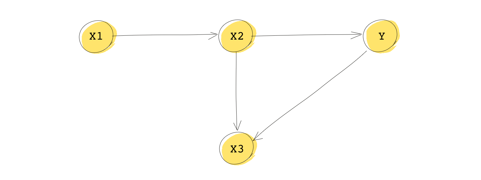
To go from $X_1$ to $Y$, there are two paths. The two paths are:

• $X_1 \longrightarrow X_2 \longrightarrow Y$
• $X_1 \longrightarrow X_2 \longrightarrow X_3 \longleftarrow Y$

Note that the direction of edges can change along a path as is the case in the second path above.

Practice

In the example above, how many paths are there between $X_1$ to $X_3$?

0

1

2

3

We can now come back to that word, acyclic (the A in DAG). Look at this example. Can you identify a path that starts from one node and ends at that very same node? The short answer is no! None of the paths in the DAG above start and end at the same node.

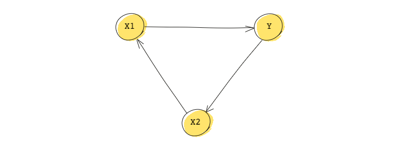
Now, consider the diagram below.

Is this a DAG?

It’s not. Notice that as you travel down the path starting from $X_1$, you eventually return right back to $X_1$. $X_1 \longrightarrow X_2 \longrightarrow Y \longrightarrow X_1$. Paths that start and end at the same node are called closed paths, they are not acylic, and therefore, any diagram with a closed path is not a DAG.

Now, one last set of terms for the road…

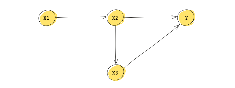
Consider the DAG we saw previously:

In this DAG:

• $X_1$ is said to be $X_2$’s parent and $X_2$ is said to be the child of $X_1$. By the same token, $X_3$ is a child of $X_2$, and $X_2$ is the parent of $X_3$. A node can have more than one child and multiple parents. For instance, $Y$ has two parents: $X_2$ and $X_3$.
• $Y$ is a descendant of $X_1$ and $X_1$ is an ancestor of $Y$.
• $X_1$ is a root. Roots are nodes with no parents.

DAGs are a bit like family trees 🌳