Pros and cons of matching

One advantage of matching is that covariate balance is addressed at the design stage of the study without consideration of the causal effect. This prevents a researcher’s biases from creeping into the process.

Matching and model independence

We don’t need to assume any functional form for the outcome model when we use matching. Remember, once we match on the covariates, we can then compare the outcomes of the matched treated and control subjects and take the average of the difference. So we don’t need to assume a specific functional form for the outcome model, unlike regression models.

After matching, even if we use a regression model for estimating the causal effect of the treatment on the outcome, the causal effect will not depend on the functional form of the regression model.

To see this, consider the following example, which is courtesy of Gary King, a Harvard political scientist and an expert in causal inference.

Imagine you are interested in the effect of going to a private college rather than a public college on future earnings. For the sake of this example, let’s also assume that parental income is the only confounder and that we can control for this variable using available data. If we decided not to use matching, we would use a regression model to estimate the causal effect. Let’s say this is our model:

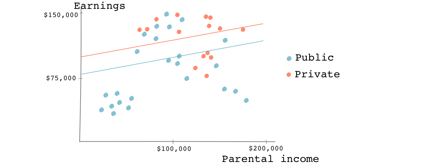
As shown in the figure below, the coefficient on the treatment variable (going to a private college) is the difference between the two regression lines; one for the treated group (private college goers) and one for the control group (the public college goers). So the causal effect is the jump from the blue line to the red line or roughly 25,000 dollars.

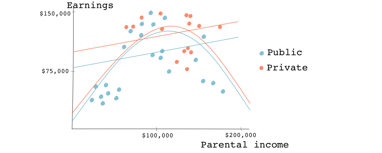
Now, let’s say a friend suggests using a regression model with a quadratic term for parental income. “Your first regression doesn’t fit the data very well. You should try using a quadratic term on the education variable,” she says. You take her advice, and now you end up with something like this:

As we can see, the effect is now smaller and almost insignificant. The newly estimated effect is represented by the gap between the two arched lines as opposed to the two parallel lines.

But why stop there? If you’ve used a quadratic term, why not use a cubic term? As we’ve just shown, the causal estimate can depend heavily on the regression model’s functional form.

But how can matching solve the model-dependence problem?

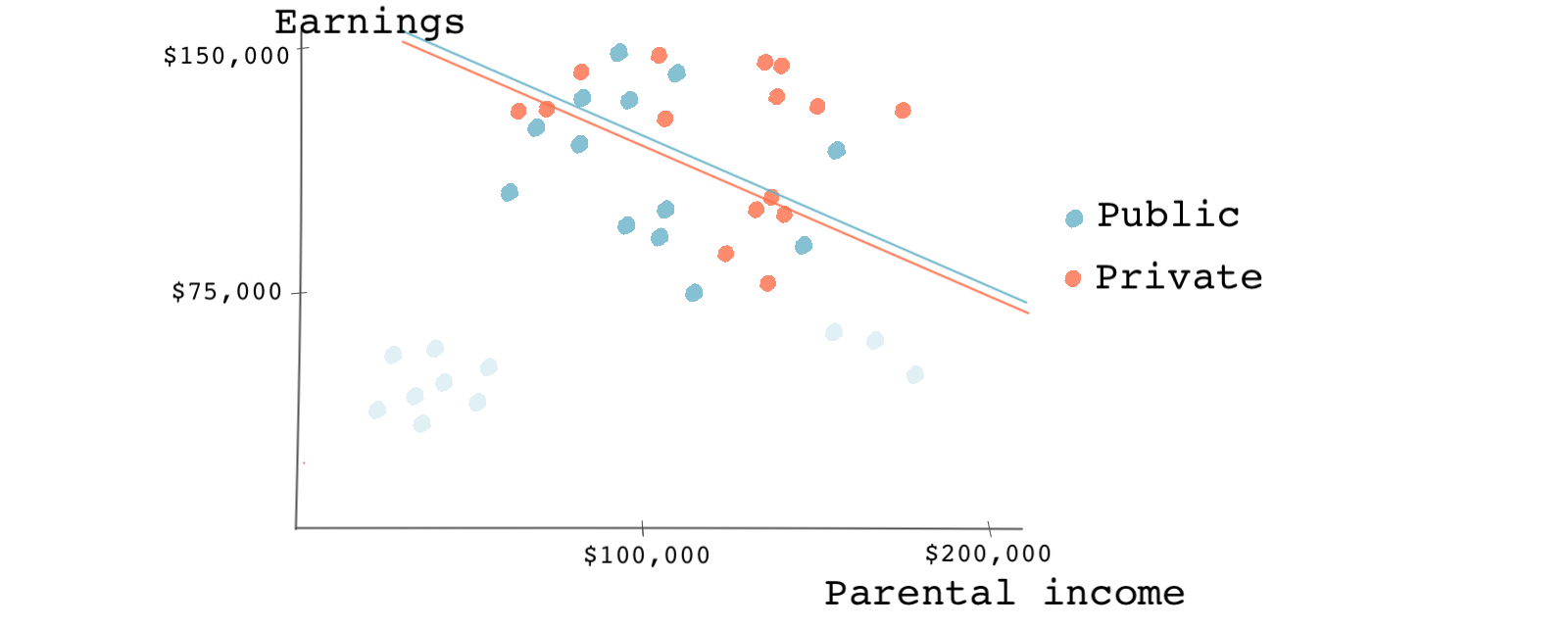
The chart below shows the results of regression after matching on our single covariate: parental income. You can see that several observations were dropped (pruned) through the matching process (the faded circles). When we use a simple regression model to estimate the causal effect on the remaining observations, we see something surprising. We now see a negative effect (attending a private college leading to lower earnings), but the difference is very small.

After matching, the causal effect should no longer depend on the functional form of the regression model. A nonlinear relationship between earnings and parental income would yield a similar small causal effect. This is because matching achieves balance for our covariate parental income. The model dependence was because of the covariate imbalance, and now that it’s gone, there shouldn’t be any model dependence.

Other advantages of matching

By looking at the covariates’ post-matching overlap or the propensity scores across the treatment and control groups, the population to which the causal estimates apply is usually revealed. If there’s a significant overlap after matching, then the causal estimates likely apply to the entire population.

If we only have a small overlapping region, the causal estimates only apply to that region’s observations. In this case, the positivity assumption does not hold for all observations. The positivity assumption ensures that every subject in the study has some chance of receiving the treatment and the treatment assignment is not deterministic. Note that this is something that a regression analysis does not specify. A regression will extrapolate the causal effect for the entire population.

In a randomized experiment, we naturally expect to have covariate balance across both observed and unobserved covariates. However, even in randomized settings, we may not have perfect covariate balance. In such cases, we can still use matching, and matching can also improve the causal effects in a randomized experiment.

The drawbacks

Despite all of these advantages, matching also has some drawbacks. Matching doesn’t work when the causal design is poor. Matching relies on the ignorability assumption, an assumption that isn’t easy to check or satisfy, as we’ve seen before. Matching doesn’t tell us what to control for. In other words, matching only improves causal estimates if our assumptions about the covariates are correct. If they are wrong, our analysis will is misguided and off-track from the get-go.

Similarly, if there are unobserved confounders, matching won’t fix the causality issues that come with the violation of the ignorability assumption. Matching only creates balance among the covariates that we match on and are, therefore, observed. Obviously, matching doesn’t improve covariates balance for unobserved covariates.

As a result, the causal effect could still be due to differences in unobserved covariates across treated and control subjects and not necessarily due to the treatment effect.

To sum up, if an important confounder is omitted from the matching process, matching fails to properly identify the causal effect, just as regression analysis would fail. Propensity-score matching is the target of a specific critique waged most prominently by Gary King and Richard Nielsen.

King and Nielsen argue that matching should be done on each covariate instead of using a propensity score. To understand this, imagine you are standing in the middle of a room full of people. You are 4 feet away from the closest person. Now, let’s prune half of the people in the room. It’s very likely that your distance to the closest person has increased. Nice, but how does this relate to propensity-score matching?

Consider an observational dataset that already replicates a randomized experiment. Consequently, the propensity scores for each observation should be roughly 0.5, as we saw earlier in this module. If we’re matching based on propensity scores, because all the propensity scores are similar, we end up randomly pruning the control observations. In the same way that randomly pruning the room full of people will make people farther from each other, pruning observations at random can make covariate balances worse.

This is especially relevant if there are covariates that we should match on exactly. Using a propensity score may actually make the covariate balance for those covariates worse.

One last note

As we saw, one of the issues with matching was that it ends up dropping observations from the sample. Besides increasing variance in the estimates, dropping observations either from the control group, the treatment group, or both changes the meaning of the causal estimates. This is also something we discussed before, but you should always keep in mind.

Nonetheless, propensity score matching is simple. It’s easier to match observations in one dimension than in multiple dimensions if we have many covariates. As it turns out, propensity scores can be used in a way that we don’t have to drop observations from our sample. In the next lesson, we’ll learn about how we can use propensity scores to give weights to each observation instead of keeping or dropping them.