Back to confounders

The common-cause criteria in DAGs

In the previous module on the potential outcomes model, we defined confounders as variables that are associated with both the treatment and the outcome. We called these criteria the common-cause criteria. We said that without considering them in causal analysis, the estimates of the causal effect might be biased. This bias is usually referred to as the confounding bias.

Now that we are familiar with DAGs we can check the common-cause criteria in a visual way. Some examples may help. In all the examples below, we’d like to check whether variable $X_1$ is a confounder. In all these DAGs, $D$ represents the treatment and $Y$ represents the outcome.

In our first DAG, let’s see if $X_1$ is a confounder!

• $X_1$ is associated with the treatment $D$ 👍
• But, it is NOT associated with the outcome $Y$ 👎

Therefore, $X_1$ is not a confounder. Now, consider a second DAG shown below:

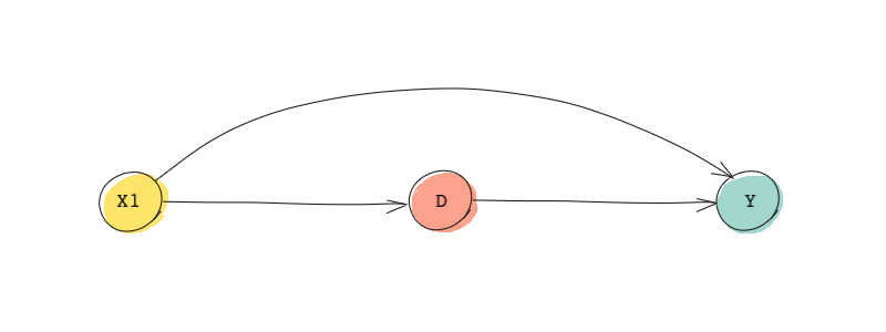
• $X_1$ is associated with the treatment $D$ 👍
• And, it is associated with the outcome $Y$ 👍

As a result, $X_1$ is a confounder based on the conditions mentioned above. Here’s another example.

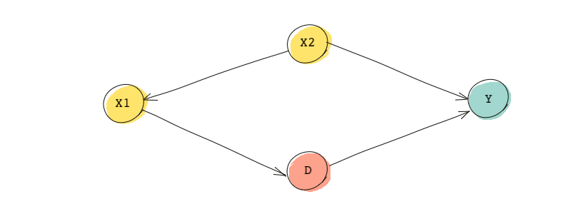
• $X_1$ is associated with the treatment $D$ 👍
• And, it is associated with the outcome through the fork originating at $X_2$ (remember that in a fork, the two end nodes are dependent on each other) 👍

Thus, $X_1$ is a confounder. Ok! One more example and we’ll be done! 😊

• $X_1$ is associated with the treatment via the fork originating at $X_2$ 👍
• And, it is associated with the outcome, 👍

Again, $X_1$ is a confounder.

A more accurate approach in identifying confounding bias

As it turns out, the common-cause criteria alone are not enough for identifying confounders. In fact, this traditional approach to causal inference (what we have followed so far) can lead to inappropriate adjustments.

It turns out we can use DAGs in a more appropriate way to identify confounding bias. To understand this, we need to learn about frontdoor and backdoor paths. We will see that to sufficiently control for confounding, we must block backdoor paths from the treatment to the outcome. If we block the backdoor path, then the ignorability assumption is satisfied. So instead of going after all confounders, we should only focus on confounders that create what are called backdoor paths.

Frontdoor and backdoor paths

Let’s first start with a frontdoor path. In a causal diagram, a frontdoor path is a path from treatment to the outcome that begins with an arrow out of the treatment and ends in the outcome. In the DAG below, if $D$ is the treatment and $Y$ is the outcome, $D \longrightarrow X_2 \longrightarrow Y$ is a frontdoor path from the treatment to the outcome.

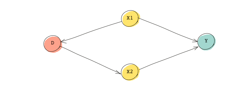
Frontdoor paths should not be blocked because they are what we’re interested in, to begin with. If a frontdoor path is blocked, then we won’t be able to see the direct effect of the treatment on the outcome.

Note that the common-cause criteria for finding confounders would tell us to control for $X_2$ because it’s associated with both the treatment and the outcome. However, if we control for $X_2$, we block the path that would give us the treatment effect itself. In the example above, if we block the frontdoor path by controlling for $X_2$, we won’t be able to find the effect of $D$ on $Y$. This is because $X_2$ partially captures the treatment.

Ok. Now that we know about frontdoors, let’s figure out what backdoor paths are. Backdoor paths are paths between the treatment and the outcome but instead of going out of the treatment, the path is directed into the treatment. In the DAG above, $D \longleftarrow X_1 \longrightarrow Y$ is the only backdoor path. Note that the path is between the treatment and the outcome and it includes an arrow going towards the treatment.

Practice

In this DAG below, the frontdoor path is simply $D \longrightarrow Y$. Which one of the following is not a backdoor path?

$D \longleftarrow X_2 \longrightarrow X_3 \longrightarrow Y$

$D \longleftarrow X_2 \longrightarrow X_1 \longrightarrow Y$

$D \longleftarrow X_1 \longrightarrow X_3 \longrightarrow Y$

$D \longleftarrow X_2 \longrightarrow X_1 \longleftarrow X_3 \longrightarrow Y$

$D \longleftarrow X_2 \longrightarrow X_3 \longrightarrow X_1 \longrightarrow Y$

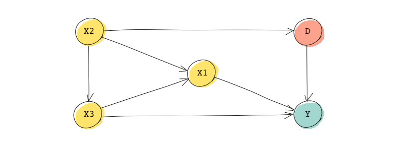
While frontdoor paths capture the effect of the treatment on the outcome, backdoor paths represent alternative paths (channels) between the treatment and the outcome that have nothing to do with the treatment effect.

In causal inference, we like to estimate the causal effect of the treatment on the outcome and not any (conditional) associations caused by other variables. Take $X_2$ in the quiz above! If we don’t control for $X_2$, some of the associations between $D$ and $Y$ will be through the backdoor paths $X_2$ is on. So to estimate the pure causal effect of $D$ on $Y$, we need to block these backdoor paths.

Practice

Michael Radelet, in his 1981 paper Racial Characteristics and the Imposition of the Death Penalty, examines the relationship between race and receiving the death penalty. Research suggests that in homicide cases, the race of the victim affects the chances of the offender being sentenced to the death penalty and that the offender’s race also affects his or her chances of being sentenced to the death penalty. Additionally, assume that the offender’s race affects the victim’s race (most crimes against whites are perpetrated by whites). The aggregate data shows that white defendants are more likely to receive the death penalty compared to blacks. However, when we disaggregate the data by the race of the victim, we find that black defendants are more likely to receive the death penalty. Which finding should we trust more?

The aggregate analysis because of the Simpson’s paradox

The aggregate analysis because of the existence of a collider

The disaggregated analysis because conditioning on the race of the victim blocks the backdoor path between the treatment and the outcome

The disaggregated data because the race of the victim is a collider and needs to be controlled for

An example

Imagine we are interested in the effect of family socioeconomic status (SES) on individuals’ income. Therefore, SES is our treatment, and income is our outcome. For the sake of our example, imagine the following DAG represents the causal relationships.

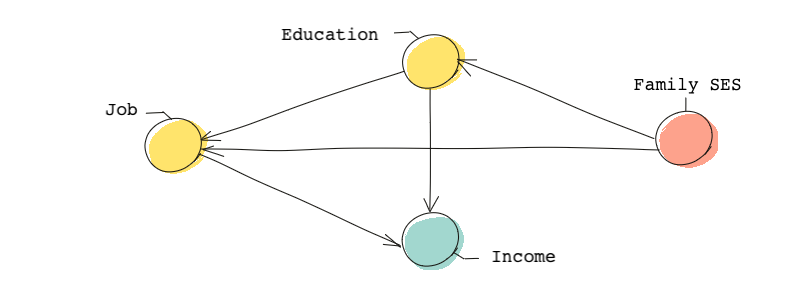
In this DAG, we need to make sure we don’t block the frontdoor path (the causal path) and we block all backdoor paths. The interesting thing about this DAG is that there are no backdoor paths. So there is no need to block any backdoor paths. But try to identify the frontdoor path.

You’ll notice that there are four!

If we control for both education and job, we will likely close all of these frontdoor paths, and therefore, we’ll be unable to establish the causal effect of SES on incomes.

We will go over what should and shouldn’t be controlled in a DAG like this soon. The main lesson here is that the common-cause criteria aren’t the best methods for identifying what we should control for. A better approach is to identify backdoor paths and to block them.