More on synthetic control

As you can see, the synthetic control method is very simple and straightforward. The method has been used to study a wide array of topics such as the effect of cigarette taxes in California or the economic cost of the unification in West Germany. The main use cases are comparative studies with small samples, one treated unit, and multiple time periods.

The weights in the synthetic control method are not model dependent, i.e., we don’t have to define a specific functional form for how they’re calculated. We also make explicit the degree to which each observation matters in our analysis by estimating a weight for each observation. In this way, the weights for observations and how they contribute to the analysis are more explicit in synthetic control studies than they are in basic regression analysis.

The limitations to the method are as follows. First, similar to matching and IPW, if unobserved confounding exists, synthetic control isn’t going to do its magic. Synthetic control finds weights based on observed confounders and not based on the ones that are unobserved.

Also, the selection of the initial donor pool is prone to all sorts of subjective bias. In some cases, researchers start with a large donor pool without a strong justification for why each control unit made the list. This is bad practice. Each unit in the donor pool should be similar, in some regards, to the treated unit. Furthermore, while it’s tempting to assume that bad donors will automatically be identified by the algorithm and assigned a low weight, by adding random control units you’ll run the risk of overfitting.

A final concern is that only the treated unit will undergo some other major structural changes during the period of study without the same change affecting the control units. For instance, imagine if the treated unit receives the treatment at time $t$ but also goes through some other major event at time $t+1$ . If this new event doesn’t affect the control units, then the effect we estimate not just includes the effect of the treatment but also the effect of the event.

Root mean squared prediction error (RMSPE)

By using the synthetic control method, we find the donor pool weights and estimate the path plots of the synthetic control unit and consequently calculate the treatment effects over time.

One of the conditions of a good synthetic analysis is that the pre-treatment outcome path of the synthetic control unit should closely follow the pre-treatment outcome path of the treated unit. But how do we quantify what we mean by “closely”?

We can’t just look at the path plots and visually decide the trends are similar or aren’t similar. Instead, we can use something called the root mean squared prediction error or RMSPE as a measure of the closeness of fit.

RMSPE measures the lack of fit between the pre-treatment path of the outcome variable for the treated unit and its synthetic counterpart. Going back to the tax policy paper, we want to find the lack of fit between the pre-treatment pollution rate between Sweden 🇸🇪 and synthetic 🇸🇪.

We say “lack of fit” because RMSPE measures the magnitude of the gap between the outcomes. Most software packages provide RMSPE but here is how it’s calculated:

\text{RMSPE } = ( \dfrac{1}{T_0} \sum_{t=1}^{T_0} (Y^{treated}_t - \sum_{j=1}^J {w^*_j Y^{control}_{jt}})^2)^{1/2}

Note that $T_0$ is the pre-treatment time interval, $J$ is the number of control units in the donor pool, and the $w$ ’s are the weights we calculated. Sometimes, people use mean squared prediction error (MSPE) instead of its root. Because RMSPE and MSPE are both used for comparison, it doesn’t really matter which one we use. But pre-treatment RMSPE isn’t enough for judging the lack of fit.

Pre-treatment RMSPE is usually used in conjunction with post-treatment RMSPE for evaluating both the goodness of fit and the size of the effect. Here’s how:

We calculate the pre-treatment RMSPE (this is an indicator of goodness of fit in the pre-treatment period)
We calculate the post-treatment RMSPE the same way (this is an indicator of the effect size in the post-treatment period)
We then divide the post-treatment RMSPE by the pre-reunification RMSPE and find a ratio.

If this ratio is large, it could be indicative of two things: the post-treatment effect is large and/or the pre-treatment fit is good. Similarly, a small ratio shows that the post-treatment effect is small and/or the pre-treatment fit is bad. By only looking at pre- or post-treatment RMSPE, we miss the big picture.

But what if the fit is poor? What if the denominator, the pre-treatment RMSPE, is large. If the fit is poor, we can go over the pre-treatment outcome trends of the treated unit and the individual donor units (not the synthetic unit) one by one. There might be a specific unit that is causing the bad fit. We can also go over the vector $V$ , the covariates weight vector, and tweak it.

Placebo tests in synthetic control

The ratio of post-treatment RMSPE over the pre-reunification RMSPE can also help us define a statistical significance test. In a typical statistical significant test, we’re interested in whether the effect size we find is random, i.e., whether the effect will continue to be large with other samples. We can use the ratio of post-treatment RMSPE to pre-treatment RMSPE to define how likely it is to find a ratio as big as the one we find for the treated unit.

Our logic for the test is this: we imagine the policy change (the tax policy imposition) didn’t happen in 🇸🇪 and instead happened in one of the countries in the donor pool such as 🇪🇸, therefore, we pretend it was 🇪🇸 that was the treated unit and not 🇸🇪. All other countries in the sample then work as a donor for 🇪🇸.

Because 🇪🇸 is not the true treatment unit, if we calculate the ratio, we expect it to be small or at least smaller than the one we found for 🇸🇪.

We then do this for another country in the donor pool such as 🇵🇱. Again, we want the ratio for 🇵🇱 to be smaller than the one for 🇸🇪. We do this repeatedly for all countries in the donor pool and compare all ratios to the one we found for 🇸🇪.

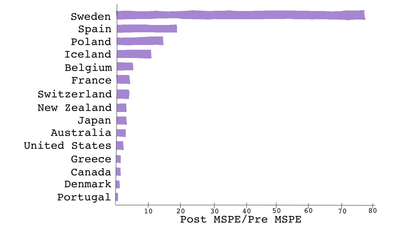
This test is referred to as the placebo test in the context of synthetic control methods and is also called a falsification or refutability test. This is shown in the plot below for Andersson’s paper.

Andersson finds the MSPE (not the RMSPE) for each country. As you can see, 🇸🇪 stands out with the highest MSPE ratio. 🇸🇪‘s MSPE is almost 5 times the next biggest MSPE ratio. Because the ratio is larger in 🇸🇪 than in the donor pool countries, there is evidence that the treatment had an effect.

Once we do the test for every donor unit, we can then have a distribution of the MSPE ratios. We can use this distribution for evaluating the estimated effect: if we were to pick a country at random from the sample, the chances of getting a ratio as high as the one for 🇸🇪 would be 1/14 or 0.07, a relatively small chance, which is good news.

Although very different in nature, the number 0.07 can be interpreted in a similar fashion as a p-value. This p-value is the fraction of an effect greater than or equal to the effect estimated for the true treated unit. These placebo-test-based p-values have very limited meaning and can’t be used to construct confidence intervals. The results of the placebo test should be treated as “suggestive” of an effect and should not be interpreted as a rejection of a null hypothesis.

# In R, you can use the outcome of the synth() function from the package Synth
# to calculate MSPE. Unfortunately, the package doesn't spit out MSPE automatically.
# The line below, estimates the gap between the treated and the synthetic units
gaps <- dataprep.out$Y1plot - (dataprep.out$Y0plot %*% synth.out$solution.w)

# This calculates MSPE for the post-treatment period
mspepost <- mean((gaps[31:46, 1])^2)

# This calculates MSPE for the pre-treatment period
mspepre <- mean((gaps[1:30, 1])^2)

# Therefore, the ratio is simply:
msperatio = mspepost/mspepre

# You can use the code above in a for-loop in order to find the ratio for each
# control unit in the donor pool.

# Python codes will be added soon

* Placebo testing
synth co2_transport_capita co2_transport_capita(1970) co2_transport_capita(1980) co2_transport_capita(1989) gdp_per_capita gas_cons_capita vehicles_capita urban_pop, ///
 trunit(13)trperiod(1990) xperiod(1980(1)1989) mspeperiod(1960(1)1989) resultsperiod(1960(1)2005)
 
preserve
* Calculating the gap between the treated outcomes and the synthetic outcomes
matrix a =  e(Y_treated) - e(Y_synthetic)
svmat double a, name(gap)
keep gap year
drop if gap==.

* Calculating the squared of the gaps
gen gap_sqrd = gap^2

* This calculates MSPE for the post-treatment period
sum gap_sqrd if year > 1989
gen mspepost=r(mean)

* This calculates MSPE for the pre-treatment period
sum gap_sqrd if year <= 1989
gen mspepre=r(mean)

* Therefore, the ratio is simply:
dis mspepost/mspepre
restore

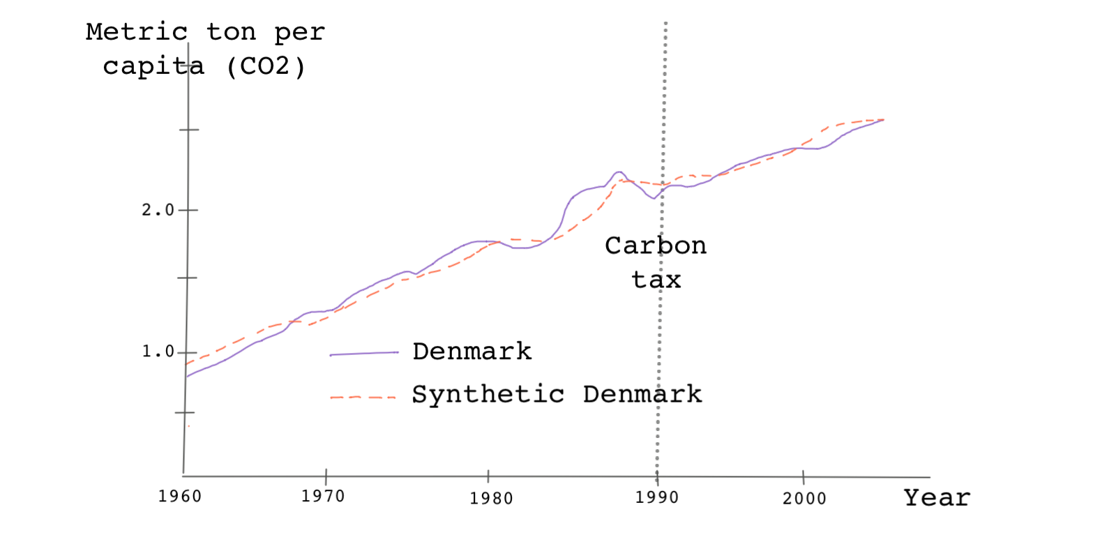
In a simpler and less rigorous version of the placebo test, we can find the control unit with the largest weight, replace it with the treated unit, and find its path plot. Then we can see how different this path is compared to the unit’s synthetic counterpart. Here, because we know 🇩🇰 has the highest weight among the donor pool countries we use 🇩🇰 as the placebo unit.

We then do the analysis as before. Notice the changes in telling the function which unit is the treatment and which units are the controls.

dataprep.out.denmark <-
    dataprep(foo = carbontax,
             predictors = c("GDP_per_capita" , "gas_cons_capita" , "vehicles_capita" ,
                            "urban_pop") ,
             predictors.op = "mean" ,
             time.predictors.prior = 1980:1989 ,
             special.predictors = list(
                 list("CO2_transport_capita" , 1989 , "mean"),
                 list("CO2_transport_capita" , 1980 , "mean"),
                 list("CO2_transport_capita" , 1970 , "mean")
             ),
             dependent = "CO2_transport_capita",
             unit.variable = "Countryno",
             unit.names.variable = "country",
             time.variable = "year",
             treatment.identifier = 4,
             controls.identifier = c(1:15)[-4],
             time.optimize.ssr = 1960:1989,
             time.plot = 1960:2005
    )

synth.out.denmark <- synth(data.prep.obj = dataprep.out.denmark)

path.plot(synth.res = synth.out.denmark,
          dataprep.res = dataprep.out.denmark,
          Ylab = "Metric tons per capita (CO2 from transport)",
          Xlab = "Year",
          Ylim = c(0,3),
          Legend = c("Denmark","synthetic Denmark"),
          Legend.position = "bottomright"
)

# Python codes will be added soon

* Using Denmark as the treated unit
synth co2_transport_capita co2_transport_capita(1970) co2_transport_capita(1980) ///
co2_transport_capita(1989) gdp_per_capita gas_cons_capita vehicles_capita urban_pop, ///
trunit(4) trperiod(1990) xperiod(1980(1)1989) mspeperiod(1960(1)1989) ///
resultsperiod(1960(1)2005) fig

Based on the plot above, because 🇩🇰 is not the true treated unit, we don’t see a divergence between the path plots after the treatment year.

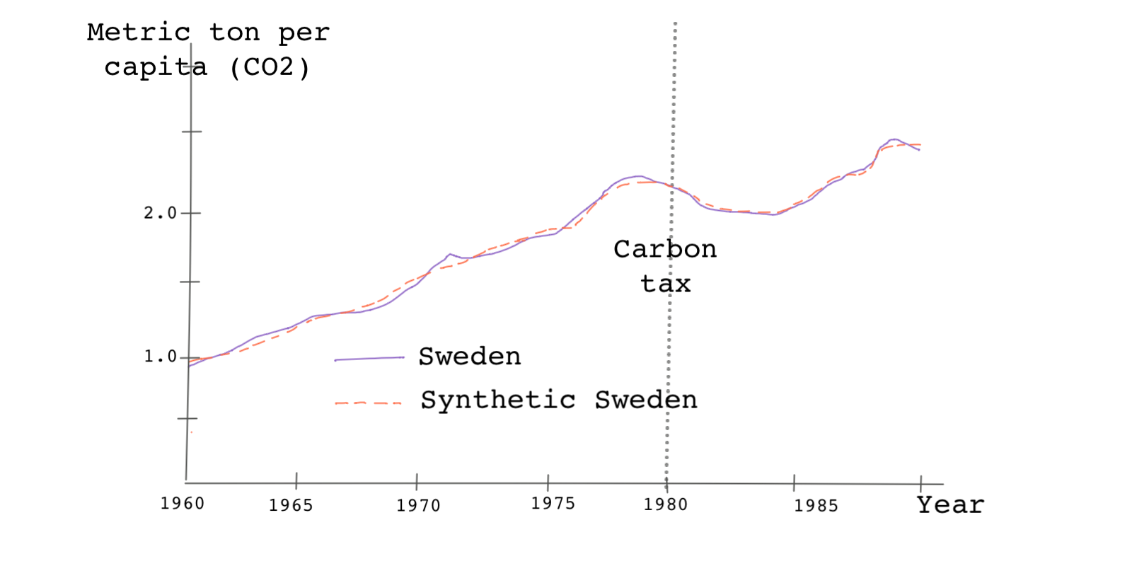
The placebo tests we discussed thus far are specifically referred to as in-space placebo tests. Another placebo test we can use, especially if the number of control units in the donor pool is small is an in-time placebo test. Remember in the Sweden tax study, the treatment happened in 1990. In an in-time placebo test, we pretend, for instance, that the treatment happened sometime before 1990 such as 1980 or 1985 or any other year.

If the treatment effect indeed happened in 1990, then we shouldn’t see any divergence between the treated unit and its synthetic counterpart in 1980 or 1985, etc.

We can do this test by simply tweaking our code so that the pre-treatment period is modified. In the following code, we specify the year of the treatment as 1980.

dataprep.out.1980 <-
    dataprep(foo = carbontax,
             predictors = c("GDP_per_capita" , "gas_cons_capita" , "vehicles_capita" ,
                            "urban_pop") ,
             predictors.op = "mean" ,
             time.predictors.prior = 1970:1979 ,
             special.predictors = list(
                 list("CO2_transport_capita" , 1979 , "mean"),
                 list("CO2_transport_capita" , 1970 , "mean"),
                 list("CO2_transport_capita" , 1965 , "mean")
             ),
             dependent = "CO2_transport_capita",
             unit.variable = "Countryno",
             unit.names.variable = "country",
             time.variable = "year",
             treatment.identifier = 13,
             controls.identifier = c(1:12,14:15),
             time.optimize.ssr = 1960:1979,
             time.plot = 1960:1990
    )

synth.out.1980 <- synth(
    data.prep.obj = dataprep.out.1980,
    method = "BFGS"
)

path.plot(synth.res = synth.out.1980,
          dataprep.res = dataprep.out.1980,
          Ylab = "Metric tons per capita (CO2 from transport)",
          Xlab = "Year",
          Ylim = c(0,3),
          Legend = c("Sweden","synthetic Sweden"),
          Legend.position = "bottomright"
)

# Python codes will be added soon

* Changing the treatment year
synth co2_transport_capita co2_transport_capita(1965) co2_transport_capita(1970) ///
co2_transport_capita(1979) gdp_per_capita gas_cons_capita vehicles_capita urban_pop, ///
trunit(13) trperiod(1980) xperiod(1970(1)1979) mspeperiod(1960(1)1979) ///
resultsperiod(1960(1)1990) fig

As you can see, the two outcome trends don’t diverge in 1980 even if we specified that the treatment happened in 1980. This evidence confirms that the treatment didn’t really happen until 1990.

Robustness tests

Because in synthetic control methods there is no rigorous way of making sure our analysis is sound, we do everything we can at our disposal to tell others our analysis is trustworthy.

Besides the in-time and in-space placebo tests we saw above, we can also perform robustness tests. Robustness tests are simple. Sometimes as simple as leaving individual donor pool units out of the analysis one-by-one and seeing how the results change.

Although by doing this we sacrifice some goodness of fit, we can evaluate the extent to which our results are driven by any specific control unit.

Next Lesson

Difference-in-differences method

You'll learn about the basics of causal inference and why it matters in this course.